Central Limit Theorem
in Data Science on Statistics

In this article, it will be explained when to use the CLT and why is so valuable. Additionally, the t-distribution is used to test the null hypothesis.
R files can be found on GitHub.
When should you use the CLT?
It’s recommended to use it when performing hypothesis testing.
Let’s say there are two data sets and it’s requested to evaluate if they are different from each other.
The null hypothesis states that they are similar to each other. No change. Therefore, it’s of interest to reject it.
Can we substract the mean of each group and capture the difference? Yes, we can.
Although, a single value doesn’t provide information about how much the result would change if the population was sampled again.
By understanding the resulting probability distribution a range of values can be provided with a confidence interval (CI).
Before continuing, let’s understand our objective better: Test our hypothesis using two independent data sets.
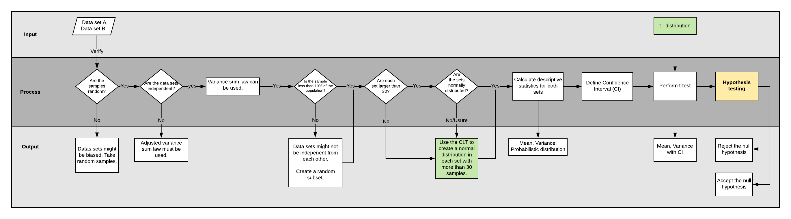
The CLT can be used when any of the below conditions are not met:
- Data set’s size is smaller than 30.
- Data set’s probability distribution is not normal or is unknown.
The t-distribution will help us provide very accurate confidence intervals based on a normal distribution given we provide its mean and standard deviation.
\[\sigma = \sqrt{\sigma^2}\]where:
\(\sigma:\) is the standard deviation.
\(\sigma^2:\) is the variance.
Here’s were the variance sum law comes into play. Mathematically, can be demonstrated that the difference in variance of two groups is the sum of their individual variances. This is true when your data sets are independent.
\[\begin{aligned} \sigma_{(X±Y)}^2 &= \sigma_X^2 + \sigma_Y^2 \end{aligned}\]What is the CLT?
Now that you know when to use the CLT, now it’s time to learn what it is exactly and how to use it.
The CLT tells us that regardless of a initial probability distribution (binomial, normal, etc) the sample distribution of the sample mean will be normal. The mean of the sample distribution of the sample mean will be equal to the original distribution. Lastly, the standard deviation will be proportionally smaller based on the sample size.
Let’s use the example below to illustrate it.
Note: The Iris flower data set (IFDS) or Fisher’s Iris data set is a multivariate data set introduced by the British statistician and biologist Ronald Fisher and will be used in the example.
The IFDS includes 50 measurements of each 3 different flower species: setosa, versicolor and virginica. Let’s focus only in the setosa and versicolor species.
Typically, a large sample size is considered when usining at least 30 samples. The histrogram of each species represent the probability distribution. A very recognizible distribution is noticeable in the histogram of the 50 samples available in the IFDS. Both species seem to follow a normal distribution in a qualitatively evaluation.

Note: both histograms are using the same scale. It is evident that each distribution will have it’s own mean \((\mu)\) and standard deviation \((\sigma)\).
This shows a beatuful nice scenario.
What if we didn’t have enough resources to measure 50 samples and/or some measurements were invalid due to errors in the measuring process?
It’s very possible that a much smaller set would be available and, in some cases, with different sizes. Will these smaller sets provide evidence of normality? Let’s figure it out!
In order to illustrate this, we will create a Setosa Set and a Versicolor Set by taking random samples of the original IFDS species respectively. The Setosa Set will have 15 random samples and the Versicolor Set will have 18.

It is very hard to know what kind of probability distribution the population has based only on these data sets.
The CLT will be used to take multiple samples of each set and calculating each subset’s mean independently. A new distribution will arise named “sample distribution of the sample mean” and it will be normal.
From the Setosa Set we will take 100 random samples of size n=5, calculate the sample mean and create a new histogram.

We have a sample distribution of sample mean that is normal. Let’s compare them:

It can be noticed that the sample distribution of the sample mean is concentrating in the mean value of Setosa Set. From here, it can be inferred that:
- the mean of Setosa Set and the mean of the sample distribution of the sample mean are the same.
- the standard deviation of Setosa Set is larger than the standard deviation of the sample distribution of the sample mean.
Now, the Setosa Set seemed to be normal already. The perceived benefit seems to be small. Let’s analyze the Versicolor Set below.

It can be observed, that the 18 random samples taken show a distribution skewed to the right. Using the CLT will help us obtain a normal distribution within the Versicolor Set.

The higher amount of sampling of sample mean, the more normal the distribution will be. In the left histogram a total of 100 samples of sample means were taken. On the right histogram, the sampling was increased to 300. In both cases, the each sample mean was calculated from a random sampling of 5 from the Versicolor Set.
By comparing both histograms can be noticed how the sample distribution of the sample mean of the Versicolor Set is now normal. It has a similar mean value and a smaller standard deviation than the Versicolor Set.

So far, we’ve done a qualitative analysis of the data sets and believed the CLT theory in regard of descriptive statistics. In the next segment, a table with the calculated values will be included in order to compare them _quantitatively.
Quantitatively demonstration
\[\mu_{Setosa} = \mu_{Setosa Subset} = \bar{\mu}_{SM Setosa Subset}\] \[\sigma_{Setosa Set} > \bar{\sigma}_{SM Setosa Set}\]where,
Setosa is the total population, N=50,
Setosa subset is a random sample from the population, n=15
Sample Means of Setosa subset, n’ = 100
Note: It will hold for the Versicolor set respectively.
Table: Setosa Means and Std Dev of Sets in cm
| Value | Setosa | Setosa Subset | Sample Means Set |
|---|---|---|---|
| n | 50 | 15 | 100 |
| \(\mu\) | 1.462 | 1.423 | 1.430 |
| \(\sigma\) | 0.174 | 0.198 | 0.093 |
Table: Versicolor Means and Std Dev of Sets in cm
| Value | Setosa | Setosa Subset | Sample Means Set |
|---|---|---|---|
| n | 50 | 18 | 300 |
| \(\mu\) | 4.260 | 4.211 | 4.201 |
| \(\sigma\) | 0.470 | 0.463 | 0.204 |
It is now both qualitatively and quantitatively demonstrated the foundation of the CLT.
Measuring the difference between Setosa and Versicolor
Now that we have two sets that follow a normal distribution, we can use the t-test to measure the difference between them and consider a confidence interval for our result.
To perform the t-test, we must use the sample means data sets for setosa and versicolor.
R has the t-test function which will be used to evaluate our hypothesis. By default, it considers a 95% confidence interval.
Result
After performing the t-test we can confirm with a 95% CI that:
The average petal length difference between setosa (1.43 cm ± 0.09 cm, n=100) and versicolor (4.20 cm ± 0.20 cm, n=300) is significantly large (2.78 cm)[2.80 cm, 2.74 cm]. (twosample t-test, p<0.001)